Tree from above, tip from below
Inside a network that grows neurons — what it knows while it grows a neuron, and whether it uses it.
A neuron’s shape is not decoration. The branching tree of dendrites that collects its inputs decides which signals it can combine, how far they travel, and how strongly they arrive at the cell body. Shape is part of the computation. That makes neuron morphology worth modelling, and it makes generative models of morphology useful: they fill gaps in reconstructions, produce realistic populations for simulations, and help tell which features of a shape actually matter.
In earlier work we trained a graph neural network to grow neurons. It doesn’t draw a neuron in one shot. It grows it the way you might sketch one: start at the cell body, the soma, then add one generation of branches at a time. At every step it answers two questions for each new tip: where does it go? and does it branch again? That is all it is ever trained to do. The neurons it grows hold up well against real pyramidal neurons from seven cell types, on the usual morphology statistics: branching patterns, branch lengths, how far the tree reaches along its main axis.

A model that does its job well invites the next question. What does the network know about the neuron while it is still growing it, and does it use what it knows? Placing one tip seems to need two kinds of knowledge: what kind of neuron this is, and what this particular tip’s surroundings look like. We went looking for both.
The short version:
- The tree, from above. The network’s first global step hands every node a summary of the whole tree. That summary does real work: take it away and the main dendrite collapses; push it along a “cell type” direction and the neuron grows more like that type.
- The tip, from below. What tells one tip apart from its tree-mates is built by message passing, not handed down by the summary: for basal tips, averaging the summary away barely changes it. The tip’s own answer forms only in the last third of the network. Pushed into one tip at every middle layer, a “long segment” direction lengthens that tip’s segment by about a third of the natural long-vs-short gap, while a random push does almost nothing and its siblings don’t move.
How the model grows a neuron
It helps to see the growing process before looking inside it.
Growth goes generation by generation. The model starts from the soma and its first branches: one apical dendrite (the main one, which in pyramidal neurons grows tall towards the brain’s surface) and several basal dendrites, without their positions. It places each of them in space and decides whether each branches into two children. The next step handles those children. We call one such round an expansion step, and the tips it handles the frontier. A neuron eight generations deep is grown in eight steps.
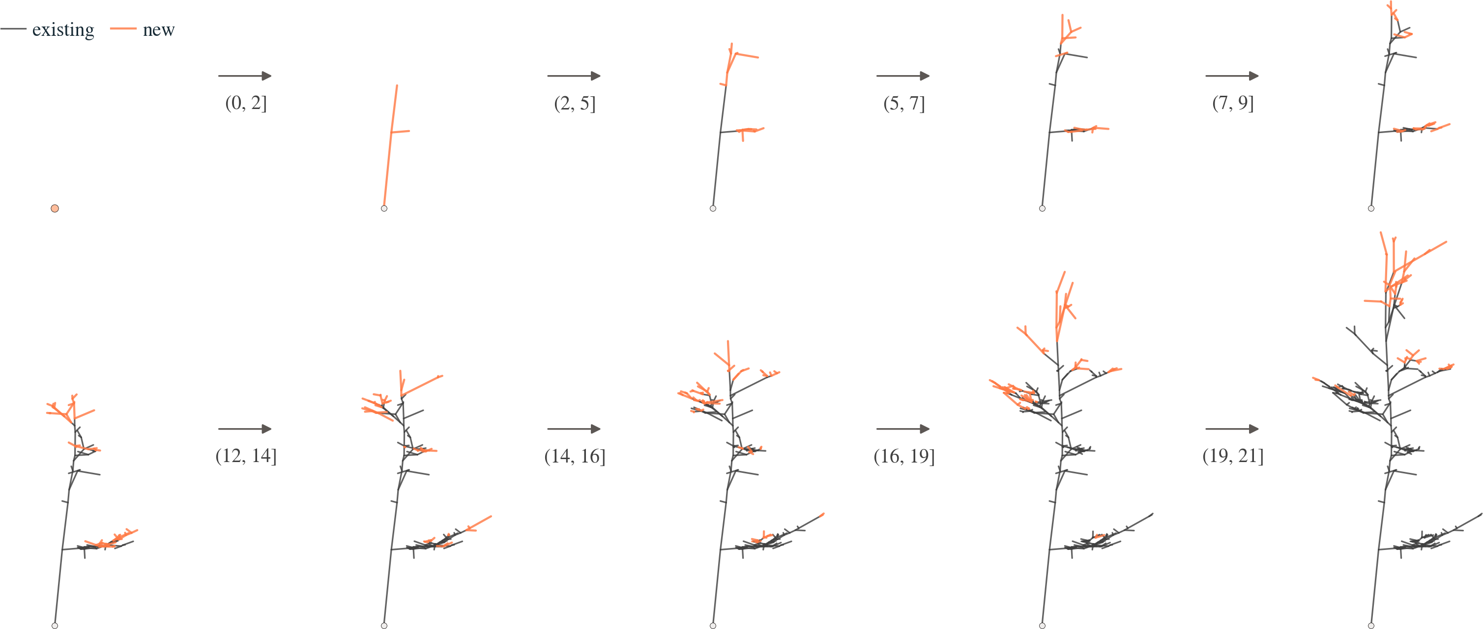
Positions come from noise. Placing a tip uses flow matching: each new tip starts at a random offset from its parent and is moved, in ten small refinement steps, towards a plausible position. The branching decision is refined the same way. One consequence matters a lot for what follows: at the very first refinement step, a new tip’s position is pure noise. Anything the network “knows” about that tip at that moment, it must have worked out from the part of the tree that is already placed. All our probes, and the node-level push in Part 2, read the network at that moment.
The network has two kinds of layer.
- Twelve message-passing blocks pass information along the edges of the tree, between each node and its parent and children. Each block moves information one hop. After twelve blocks, a node could in principle hear from anything twelve branches away.
- Every other block also has global attention: eight learned tokens read all the nodes of the tree, and each node then reads back from the tokens. This is the network’s main shortcut between distant parts of the tree, which matters, because two tips on different dendrites are connected only through the soma, often more than twelve hops apart. (A weaker second route: each block’s layer norm uses statistics computed over the whole tree.)
Geometry enters only through the edges (lengths and angles between connected nodes), so nodes carry no absolute coordinates. The model is also told which primary dendrite is the apical one: the first branch of the soma carries a flag.
Every step starts from scratch. The network keeps no memory between expansion steps. Each step runs it fresh on the tree grown so far, and the only thing passed forward is the tree itself: where the tips were placed and which of them branched.
Naming the checkpoints. “Layer” below always means a layer of the network within one step, not a generation of the neuron. We read the network at L0 to L11, the node states after each block, and A1, A3, …, A11, the node states right after a global step. The order at the start is L0 → A1 → L1, so A1 is the first point where every node has heard from the global tokens, and L1 is the first point where a new tip has heard from two hops away.
Part 1. The tree, from above
Finding the summary: a jump that looked like node knowledge
The standard tool for looking inside a network is a linear probe. Take a node’s internal state at some layer (here a 256-number vector), fit a linear model that predicts some property of that node (say, how big its subtree will eventually be), and test it on neurons the probe has never seen. If the property can be read off linearly, the network holds it in a form that later layers can easily use. We score probes by rank correlation, \(\rho\): does the probe order the nodes the way the truth does?
Our first probes showed a striking pattern. Right after the first global step, at A1, what each node seemed to know about itself jumped. Take a tip’s distance from the soma along its branch. For tips seven or eight deep, nothing about it is readable from the input (\(\rho = -0.02\)), yet right after the first global step it is readable at \(\rho = 0.60\) (untrained network: 0.05), before a single message has travelled more than one hop. It looked as if every tip suddenly knew where it was.
It didn’t. The global tokens were telling every node what kind of tree it was in.
A toy example shows the trap. Take two neurons. In the first, the nodes sit 10 to 12 µm from the soma; in the second, 50 to 52 µm. Now imagine a “probe” that knows nothing about any individual node, only each tree’s average distance, and predicts that average for every node. Pooled across both trees, it scores a rank correlation of 0.88. It knows which neuron each node is in, and that is enough. Real neurons behave the same way. For tips five or more branches deep, three quarters or more of the spread in soma distance lies between neurons rather than within them. Big neurons have tips far from the soma.
The fix: score within the tree. Before measuring rank agreement, we subtract each tree’s average from both the true value \(y\) and the prediction \(\hat y\):
\[\rho_{\text{within}} = \operatorname{Spearman}\big(y_i - \bar y_{g(i)},\; \hat y_i - \bar{\hat y}_{g(i)}\big),\]where \(g(i)\) is node \(i\)’s tree. Anything shared by the whole tree now scores exactly zero. To win, a probe has to rank nodes within a neuron: this tip’s branch will grow more than that one’s.
Rescored this way, the A1 jump vanishes: the within-tree score for soma distance at A1 is \(-0.01\). The same holds for every node property we probed: right after the first global step, nothing about a node’s own place is linearly readable, only facts about its tree. This doesn’t mean every node receives an identical message. Each node sends its own query to the tokens, so what comes back can differ. But whatever differs doesn’t encode any of the node properties we looked at, at least not linearly.

A1 the pooled score jumps to 0.60 while the within-tree score stays at −0.01. The within-tree score only rises at L1, when messages from the tip’s neighbours arrive.A second shared label, hiding in the inputs. The model is told which dendrite is the apical one, and that flag is set from the finished neuron. Apical dendrites grow far more than basal ones, so “I am on the apical”, copied down the dendrite by message passing, predicts a lot of a node’s future on its own. In our first probes it explained most of what looked like foresight about a tip’s future: restricted to basal tips, the last layer’s \(R^2\) for future height fell from 0.34 to 0.06.
What the summary contains
For whole-tree properties the right probe isn’t per node: it is one row per partial tree, reading the tokens and the tree’s average node state.
After the very first global step, the summary already encodes the tree’s overall shape: the tallest dendrite’s reach is readable at \(R^2 = 0.92\), against \(0.76\) for the untrained network (the same architecture with random weights). Cell type is the more striking case. From a partial tree only four generations deep, the network’s state predicts the neuron’s type at balanced accuracy 0.48, above the untrained network (0.44) and not far below a classifier given the finished neuron’s full branching pattern (0.55). Four generations in, the network has a fair idea of what it is growing.
Is the summary used?
Probes only show that information is there. A network can carry plenty of information it never acts on. To see whether growth actually uses the tree summary, we intervene while the network grows neurons.
How we asked. Grow the same neuron twice: once normally, and once with the global write replaced. Normally, the tokens read the tree and send each node its own message. In the edited run, each node instead receives one of two averages:
- the dataset average: the same generic message for every node of every tree. This removes everything specific to this tree.
- its own tree’s average: the mean of the messages to all nodes of the tree grown so far, recomputed at every pass. Every node in the tree gets the same message, so this removes only what differs from node to node.
For a fair comparison, both runs must start every new tip from the same noise. That is harder than it sounds: if the edited run grows one tip more or fewer, a shared stream of random numbers shifts by one, and every later tip receives its neighbour’s noise. So we tie each tip’s noise to its place in the family tree (“second child of the first child”, and so on). A tip that exists in both runs then starts from identical noise, and any difference that remains is caused by the edit. With the edit switched off, the two runs are bit-identical.
How we judged. The paired difference over a set of neurons, \(\Delta = \operatorname{mean}_{\text{neurons}}\big(m(\text{edited}) - m(\text{normal})\big)\), for three readouts:
- apical reach: how far the main dendrite extends along the cell’s main axis;
- neurons with two or more tall arms: the share of neurons where at least two dendrites each reach 60 % of the tallest, a failure mode where two dendrites compete to be the apical. In real neurons this happens 20 % of the time;
- realism: the MMD, a distance between the morphology statistics of generated and real neurons. Lower is better.
| what each node receives from the tokens | apical reach | neurons with ≥ 2 tall arms | realism (MMD) |
|---|---|---|---|
| normal | 248 µm | 17 % | 0.061 |
| the dataset average | 113 µm (−55 %) | 69 % | 0.279 |
| its own tree’s average | 297 µm (+20 %) | 8 % | 0.062 |
The summary is needed. Without tree-specific global information, the apical loses half its height and most neurons sprout two competing “apicals”. Basal reach drops by about 20 %, so the summary matters most for the trunk.
We should be careful with the third row. Give every node just its own tree’s average and realism is restored, which could be read as “the summary holds all the useful signal”. But realism is judged on whole-tree statistics, the same morphometrics we judge generated neurons on, and not on errors in individual placements. What the table does show is that the network builds this summary quickly and leans on it, even though its task is local: placing tips and deciding whether they branch. Part 2 asks what else goes into those local decisions.
Two smaller observations. Removing the global write in only one pair of blocks has far smaller effects than removing it everywhere: the blocks back each other up, so this is a property of “the global read” rather than of any one layer. And with only the tree average, the apical grows a bit taller than normal (+20 %), and two-tall-arm neurons drop to 8 %. This is the node-specific part of the global read: each node sends its own query to the tokens, so what comes back can differ from node to node. At A1 that part encoded none of the node properties we probed, yet removing it in every block still changes growth: the apical grows taller.


Steering the tree-level state: cell type
If a tree summary guides growth, can we steer it?
How we asked. For each of the seven cell types \(c\), take the direction between the average network state of trees of that type and of all other trees, \(v_c = \mu_c - \mu_{\neg c}\), comparing trees grown to the same depth (whether a push just makes neurons bigger is checked by the size-blind classifier below). Then, while the network grows a neuron, add it to every node at one layer, at every step: \(h \leftarrow h + \alpha\, v_c\), with \(\alpha = 1\) meaning one typical difference between the groups. Adding the same vector to every node shifts the tree-level part of their states, the part all nodes share; it doesn’t touch the global tokens themselves.
How we judged. A classifier trained on real neurons’ morphology: does the probability of type \(c\) rise, and more than for any other type? Cell types differ in size, so we also use a version of the classifier that cannot see size at all. A push that only makes neurons bigger fools the first classifier but not the second. Both are simple logistic regressions on morphometrics, so they are a coarse judge of type: we read them for the direction of the change, not as a measure of how convincing the steered neuron is.
It works, for the most part. Every one of the 28 conditions (seven types, four layers) raises the pushed type’s probability under the full classifier, and 26 of 28 under the size-blind one. Pushing at L7, in the middle of the network, the pushed type gains more than any other type for six of the seven types. Rare types move a lot: the average probability of layer-5 near-projecting neurons rises from 2 % to 27 %. Deeper pushes move the neuron harder but cost realism, while early pushes keep neurons realistic but are weaker and less specific.
The failures are informative too. Pushing any one of the three layer-5 subtypes (intratelencephalic, extratelencephalic, near-projecting) also raises the other two. That could mean they genuinely share morphology, or that the network has a shared internal code for them; this experiment can’t tell which.

L7 (α = 1) towards the layer 2/3, layer-5 near-projecting and layer-6 intratelencephalic types, with the same noise; the apical in red. Typical examples, not the strongest.Part 2. The tip, from below
The summary tells every node what neuron it is in. Placing a tip needs more: what tells this tip apart from its tree-mates. So from here on every score is within-tree, and two more checks apply.
- The untrained network. The same architecture with random weights also passes structure along. Message passing averages over neighbours whether or not it has learned anything, and global attention averages over the tree. So every claim below is “beyond the untrained network”, not “beyond zero”.
- Depth five or more. Near the soma, local facts come for free. A tip three branches deep is two hops from the first branch of its dendrite, so it can know that dendrite’s reach after two message-passing steps without working anything out. Five branches deep, that information is four hops away. So we use tips at least five deep.
The question for this part: is that node-level information built by message passing, or handed down by the summary? Two pieces of evidence point the same way: when it appears, and what happens to it when the summary is averaged away.
When node-level information appears
A new tip’s own position is still noise, so the nearest real geometry is its parent’s segment. It reaches the tip at exactly the first layer where it can: at L0 the parent receives a message along its own segment, and at L1 the tip receives a message from the parent. The within-tree score for the parent’s segment length goes from \(\rho = 0.02\) at the input to \(0.80\) at L1 for tips five or six deep (untrained network: 0.32). This is less a finding than a check that the probes see information arrive hop by hop.
Features of the wider neighbourhood also start to appear at L1, and then sharpen slowly over the middle layers. The untrained network reads part of them too, since random message passing still mixes each neighbour’s geometry into the tip’s state, but it doesn’t sharpen them, and loses them with depth (tips five or six deep, within-tree \(\rho\)):
| feature of the tip’s surroundings | trained, L1 | trained, best (layer) | untrained, L1 | untrained, same layer |
|---|---|---|---|---|
| the parent’s branch angle | 0.65 | 0.82 (L8) | 0.39 | 0.35 |
| how the parent’s segment points relative to the soma | 0.57 | 0.72 (L11) | 0.38 | 0.28 |
| whether the parent runs along the local subtree’s main axis | 0.21 | 0.40 (L11) | — | — |
Facts that need comparing across dendrites are never computed: basal tips have essentially no idea how their dendrite ranks against the other basal dendrites (\(\rho < 0.1\); untrained network ≈ 0).
What bears directly on the objective forms last: where the tip’s new segment goes. For tips seven or eight deep, the length of that segment is barely readable for the first half of the network (\(\rho \approx 0.04\) up to L5, 0.06 at L7), then climbs to 0.15 at L9 and 0.25 at L11; the untrained network stays at zero. It weakens with depth (0.28 for tips five or six deep, 0.12 for tips thirteen or more deep), as if deep tips lean more on the scale of the tree. The tip’s own bend follows the same late rise but stays weak (0.18 for tips five or six deep, near zero for the deepest).

L1, when no message from the parent has reached the tip. The parent’s segment arrives at L1; the parent’s angle, direction and alignment with the local subtree arrive at L1 and sharpen; a basal dendrite’s rank is never computed; the tip’s own new segment forms last.Built from below, not handed down
The network could, in principle, use the global summary to read its local cues: “in a neuron like this, a parent segment like that means a long child”. Scoring within the tree already removes anything the summary hands to every node alike, but not everything: each node queries the tokens with its own state, so some node-specific information can still come back through the global read (Part 1). To close that route too, we repeat the probes with the global write replaced by its dataset average in every block, a similar edit to Part 1’s (here the average is taken over stored states at the first refinement step), and refit them.
The late build-up survives. For tips five or six deep (on the tips this comparison uses, which differ slightly from those above, hence 0.34 rather than 0.28), the within-tree score for the tip’s own segment length is the same with and without the summary up to L7 (0.17 vs 0.18); only in the last layers does a gap open, ending at 0.34 normally and 0.29 without. The tip’s own bend is unchanged (0.18 vs 0.19), so the angle, too, is local, just weakly readable, and so are the cues both are built from (the parent’s segment: 0.84 normally, 0.89 without the summary).
Where the summary does add to the node level is the apical. Basal tips barely change on either score (0.33 vs 0.31 within the tree, 0.17 vs 0.17 within the dendrite), so the late gap above comes from apical tips. That matches how apical tips use the summary in the first place: for tips five or six deep, half of an apical tip’s final pooled score for its own segment length is already there right after the first global step, and none of it survives scoring within the tree: it comes from knowing which neuron the tip is in. Within the tree, apical tips build less (0.02 to 0.15) than basal tips (to 0.32). Apical tips carry the apical flag, and the summary already knows the apical’s reach. It fits Part 1, where removing the summary cost the apical 55 % of its reach and basal dendrites 20 %.
One caution: the edit pushes the network off its normal inputs, so the ablated states are not ones it was trained on. That the probe fitted on normal states reads them about as well as a refitted one suggests the information sits in the same place.
A glimpse of the future
In the same late layers, a basal tip’s state also starts to rank how far its branch will eventually grow, though nothing in the task asks for it: for basal tips five or six deep, scored within their dendrite, future path length rises from 0.18 at L5 to 0.38 at L11 (untrained network: 0.01). For these tips it also survives averaging the summary away. We read it as a by-product of deciding the present, and don’t test whether it is used.
Is it used? Pushing one tip
Probes show that a tip’s state carries a ranking of its own segment length within its tree. That doesn’t mean the network reads it from there. As with cell type in Part 1, we push the state and watch the output, but now into one tip only.
How we asked.
- The direction. The probes above showed that a “long segment” signal exists in a tip’s state. To push it, we build the direction directly from the data. Within each partial tree, split tips five or more deep into those whose real segment ends up long and those whose segment ends up short (top vs bottom third), and take the difference of their average states. Averaging these within-tree differences gives a “long segment” direction that carries no tree-level information by construction. The direction is fitted on one set of neurons and pushed on another.
- The push. In each partial tree, pick one apical and one basal tip (by a fixed seeded hash, not by their values) and add \(\alpha\, v\) to its state only, where \(\alpha = 1\) is the natural distance between long and short tips.
- The readout. The length of the network’s first estimate of that tip’s new segment, at the first refinement step. At that point the estimate is an average over possible endpoints, so it is shorter than real segments, and it also grows if the network becomes surer of the direction. We compare it with the same pass without the push. The noise is identical, so any change is the push. We also read the tip’s siblings and the rest of the tree.
- The scale. The network’s own predictions differ by 0.30 in log length between long and short tips within a tree. That is the gap a push has to be measured against.
Pushed at every middle layer, from L5 to L10, at \(\alpha = 1\) the target tip’s predicted log length rises by 0.11 for apical tips and 0.09 for basal tips, about a third of the natural long-vs-short gap. A random direction twice the size, pushed on the same schedule, moves it by −0.01 (apical) and +0.02 (basal). The siblings move by less than 0.001: the effect is local to the tip we pushed. About half of it comes from the last pushed layer alone (+0.06 when pushing at L10 only).
| push into one tip | Δ log length, apical | Δ log length, basal |
|---|---|---|
“long segment”, every layer L5–L10, α = 1 | +0.11 | +0.09 |
“long segment”, L10 only, α = 1 | +0.06 | +0.06 |
random, every layer L5–L10, α = 2 | −0.01 | +0.02 |
The same push for the tip’s bend moves the bend similarly.
What a reader should take, and not take, from this:
- The persistent push gives a yes: a within-tree, node-level direction, built from the data and pushed into one tip, changes that tip’s answer in the expected direction, and nothing else in the tree moves.
- The direction isn’t purely about length: the same push also nudges the tip towards branching.
- This is teacher-forced. It reads the network’s estimate of the final position at the first refinement step, where later refinement can’t dilute the push. Showing the same effect in a generated neuron would need the push at every refinement step.
- The numbers come from 512 held-out neurons (2,006 apical and 536 basal target tips); the basal estimates are noisier.

L5–L10, α = 2 (red), with the normal estimate in light blue underneath. This is a larger push than in the table (α = 2, and all basal tips rather than one) so that the change is visible: basal segments come out about 17 % longer.What we take from it
At every step, the network first tells each node what neuron it is in. That summary does real work: it sets the trunk, and editing it moves the neuron’s cell type. The rest of the step is about the individual tip, and it is built from below: the geometry next door arrives in the first layer, the wider neighbourhood sharpens slowly, and the tip’s own answer forms at the end, mostly without help from the summary. That node-level information is not just present: pushed into one tip over several layers, it changes that tip’s answer and nothing else.
Three practical lessons carry over to anyone probing models of graphs, molecules, meshes or scenes:
- Separate the levels. Score node-level probes within the instance, or you will mostly measure which instance a node belongs to. What is shared across the instance isn’t noise: here it was the most important part, the trunk.
- Always compare against the untrained network. Averaging layers produce surprisingly readable structure before learning anything.
- Audit the inputs for labels derived from the answer. Our apical flag was set from the finished neuron, and it quietly explained most of our first “look-ahead” result.
Limits
- Probes show presence, not use. Our interventions test the tree summary, cell type and the tip’s own segment length. For everything else, including the glimpse of the future, we only see it forming.
- Linear read-outs. A low score means “not linearly readable”, not “absent”. In particular, the node-specific part of the global message may carry information our linear probes don’t see.
- Teacher forcing. Probes and the node-level push see true partial trees at the first refinement step, not the model’s own generations. The summary interventions run on the model’s own generations, which partly closes that gap.
- Ablations are off-distribution. Replacing the global write with an average feeds later layers inputs they were never trained on.
- Modest absolute numbers. Within-tree scores of 0.2–0.3 are real but not large.
- Scope. One model, one dataset of cortical pyramidal neurons, one untrained control.
Methods in brief. 26,469 reconstructed pyramidal neurons of seven types. Probes are linear, fit with cross-validation grouped by neuron on 2,529 validation neurons, and read at the first refinement step, where each new tip’s position is pure noise. Node-level results use tips at least five generations deep, scored within trees, and are compared against the same architecture with random weights. Interventions grow each neuron twice with noise tied to each node’s lineage and compare the pairs. Node-level directions are fitted on held-out neurons.